Graphics in MATLAB - Basics

Introduction

Graphical representation of problems is very important in engineering problem solving. Plotting the results usually leads to additional insight into the nature of the problem.  So plotting is an important element to use and become skilled at using with MATLAB.

MATLAB has an excellent set of graphic tools.  Plotting a given data set or the results of computation is possible with very few commands.  You may need multiple plots to occur in a single window, or multiple windows to plot your functions.  You will be able to label the axis, label the graph, choose colors and symbols for the plot, or use the default axis and colors.  If you have created a plot, and then enter a second plot command, the first plot will be overwritten unless you type some special commands to keep the current plot or create a second Graphics Window.

Basic Plotting

The MATLAB command to plot a graph is plot(x,y). A graphics window with a plot of vector y versus vector x appears in response to this command. For each element of vector x, a yvalue must me defined (both x and y are either row vector s or column vector s of the same length).

Example

>>x=linspace(0,4*pi,100);

>>y=sin(x);

>>plot(x,y)

Figure 1 Plot for the vectors x and y=sin(x)

If y is a vector, plot(y) produces a piecewise linear graph of the elements of y versus the index of the elements of y. (In this example there are 100 elements in the vector y)

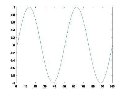
Figure 2: Plot for the vector y

The Plot Command

The syntax for linear plot command is

plot (x, y, ‘color style marker’, ‘PropertyName’, PropertyValue )

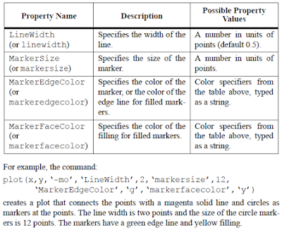
The color, style and marker values are optional to define the properties of the line. The color of a single curve is, by default, blue. If required these properties are typed inside a single quote. The letters used to define each property is given Table 1 below. Also the PropertyName and PropertyValue parameters are optional and are used to specify the line width, marker size and edge, fill color, etc. First type property name in quote marks and type the value after a comma. The list of available properties is given in Table 2.

Table 1 - Color Marker Style Properties and Codes

 

Table 2 - Other Plot Properties

Example

>> plot(x,y,'mx:')

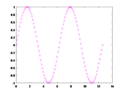
Figure 3 - Plot with Color-Magenta, Marker-x and style dotted

>> plot(x,y,'gh-.')

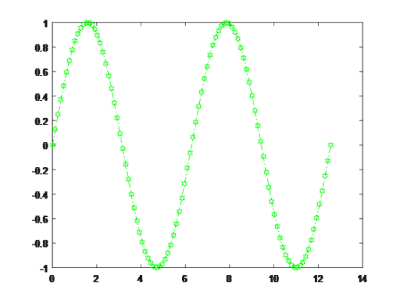
Figure 4 - Plot with Color-Green, Marker-hexagon and style dash-dot

Adding Title, Axis Label, Legend,…

Title, labels, etc. can be easily added to the plot using simple commands. The common commands are listed below.

X-axis label.

 xlabel('text') adds text beside the X-axis on the current plot.

Y-axis label.

ylabel('text') adds text beside the Y-axis on the current plot.

TITLE

title('Some text') writes title above plot

TEXT

text(x,y,'Some text') places text in figure with first character at (x,y)

LEGEND

legend('text1','text2',...) writes legend - For each graph (data set) displays short line in same style as graph line and adds specified text.

Example

>> x=linspace(0,4*pi,100);

>> y=sin(x);

>> plot(x,y)

>> xlabel('x (secs)')

>> ylabel('sin(x)')

>> title('plot of sine function')

>> text(pi,0,'zero crossing')

>> legend('sine')

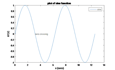
Figure 5. Plot with title and labels

Plot Two or More Curves on Same Window

More than one plot can be drawn on the same figure window.  This can be done in different ways. 

The hold command can be used to keep the existing graph and draw a new curve on the same figure window.

hold on - holds the current plot and all axis properties so that subsequent graphing commands add to the existing graph.

hold off - returns to the default mode

hold - toggles the hold state.

Example

>> t=linspace(0,2*pi,100);

>> x= sin(t);

>> y= cos(t);

>> z= tan(t);

>> plot (t,x)

>> hold on

>> plot(t,y)

>> legend('sine','cose')

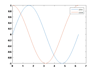
Figure 6 Multiple plots using HOLD command

Multiple (x, y) pairs arguments can create multiple graphs with a single call to plot.

plot(x, y, u, v, t, h)plots y vs. x, v vs. u, h vs. t. Vectors of each pair must be same size but can be different than sizes in other pairs.

Example

The curves in the previous example can be plot by

>> plot(t,x,'-b', t,y,'--r',t,z,'g:')

>> xlabel ('time')

>> ylabel('trignemetric functions')

>> title('Multiple curves in a plot')

>> legend('sine(t)','cose(t)','tan(t)/10')

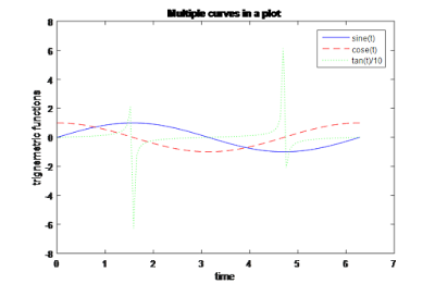
Figure 7. Typical example of multiple plots using single plot command

Line(x,y) commandadds additional lines in vectors x and y to an existing plot. The x,y pair can be followed by parameter/value pairs to specify additional properties of the lines.

line(x,y,'PropertyName','PropertyValue')

Example

>> plot (t,x)

>> line(t,y)

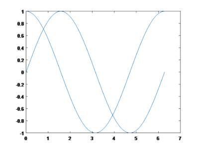
Figure 8. Example of use of line command (Note: line command use the default color if not specified)

subplot(m, n, p)  command can be used to break the figure window into an m-by-n matrix of small axes and draw different curves in each section  specified by third argument p.

Example

>> x=-10:10;y=x;z=x.^2;s=x.^3;k=10.^x;  

>> subplot(2,2,1), plot(x, y)

>> subplot(2,2,2), plot(x, z)

>> subplot(2,2,3), plot(x, s)

>> subplot(2,2,4), plot(x, k)

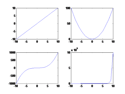
Figure 9. Subplot example